3 Tidyverse

The goal of this Tidyverse section is to learn

• Subsetting Datasets
• Merging Datasets
• Summarizing
• Plotting

In this section we will be continuing to be working with the BLS data we downloaded in the Introduction.

Tidyverse provides us with some useful tools for data manipulation and cleaning. I include examples and descriptions of the commands I have most frequently used.

3.1 Filtering with Pipes

indiana<-                                    # 1
    unemp_data %>% filter(State_fips=="18")  # 2

What is going on in this line of code? Let’s start with the second line. The operator %>% is called a pipe. This comes from a package called magittr which is included within tidyverse. Pipes are very handy for neatly writing longer sequences of code. Here we begin with a pretty simple example. We can think of pipes as saying “then.” That is it takes the argument before it and uses it as input in the following command. Here we are using a filter command, so we are saying take our data.frame county_data, then filter or “give us” the values where State_fips is equal to “18” (this is fips code for Indiana. Go Hoosiers!). So in summary we are just filtering out indiana data and saving it as a new data frame (this is line 1). Note: this operation does NOT impact county_data, the only way we ‘over write’ a data frame is to explicitly tell it to. For example the following WOULD overwrite county_data.

unemp_data<-unemp_data %>% filter(State_fips=="18")  # 1

3.2 Plotting Data

In this lesson we will be plotting the data gathered in previous lessons. ggplot2 is a very popular package for plotting and is now included as part of the tidyverse package. It allows us to make many different kinds of plots and customize them. As it is so popular there are many guides for it. Tidyverse’s website summarizes some very useful resources.

As ggplot2 has so many options, we will just be barely skimming the surface in this introduction. Let’s start with a minimal command. First let’s load in ggplot2 filter our data down into just Indiana.

library(ggplot2)                                    # 1
                                                    # 2
indiana <- unemp_data %>% filter(State_fips=="18")  # 3

ggplot(data=indiana, aes(x=Year, y=Unemp_rate,   # 1
    colour=County_fips, group=County_fips))+     # 2
  geom_line()                                    # 3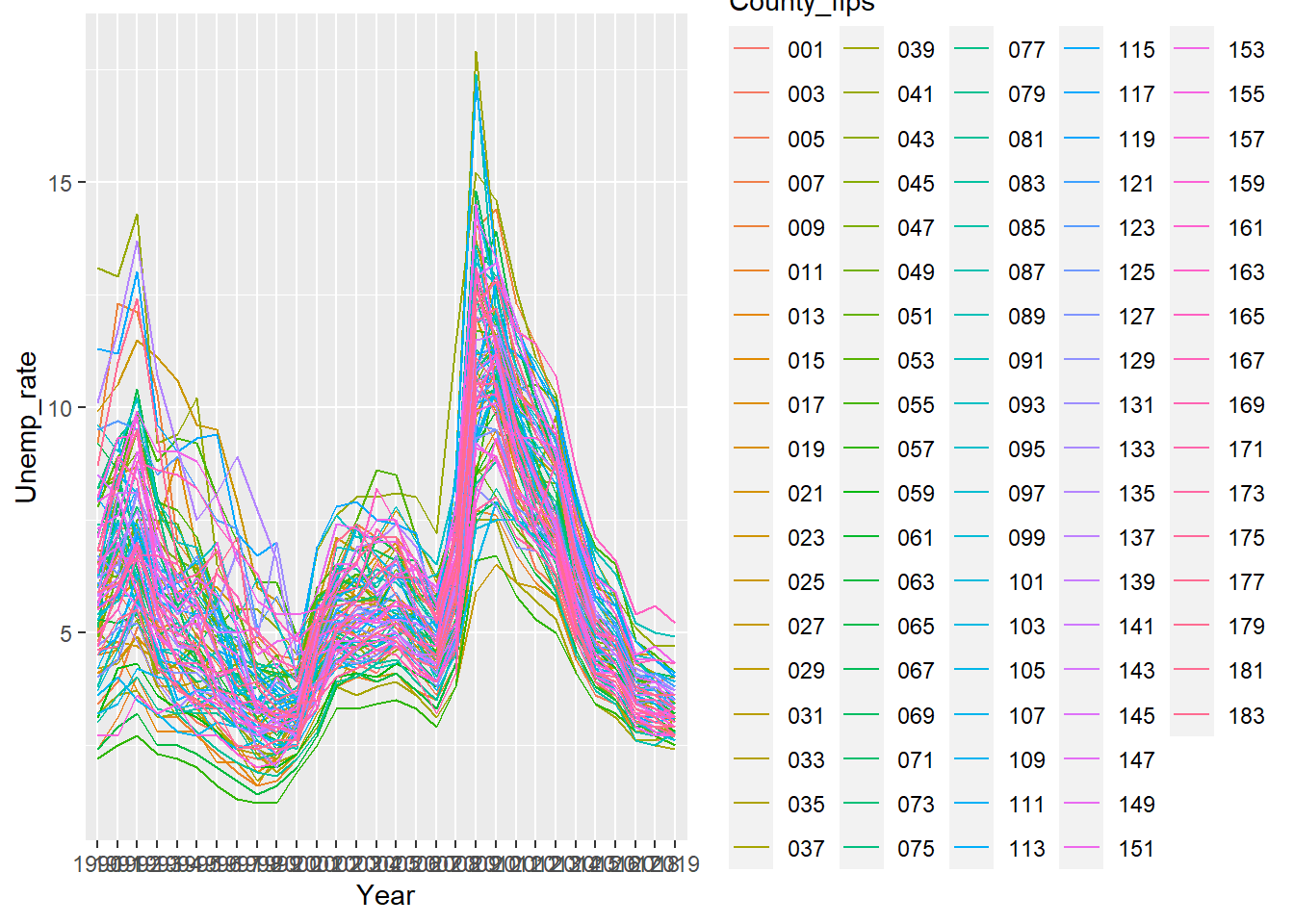

• Line #1: Tells ggplot we will be using the data.frame indiana. aes is short for aesthetics. This is where we tell ggplot how to map our data into the plots. Here I want ggplot to plot Year on the x-axis, Unemp_rate on the y-axis.
• Line #2: A continuation of the aesthetic mapping, his line is saying plot separately for each County_fips separately, giving them a different color.
• Line #3: Tells ggplot to plot the data as lines.

First thing after this plot, the legend is excessive. Let’s just suppress it for now. To do this we can define the legend.position in theme as none. The theme command allows for a lot of customization with the plot. If you want to see all options click here. Let’s also change the thickness of the lines, we can do this with the alpha argument.

ggplot(data=indiana, aes(x=Year, y=Unemp_rate,   # 1
    colour=County_fips, group=County_fips))+     # 2
  geom_line(size=0.3)+                           # 3
  theme(legend.position="none")                  # 4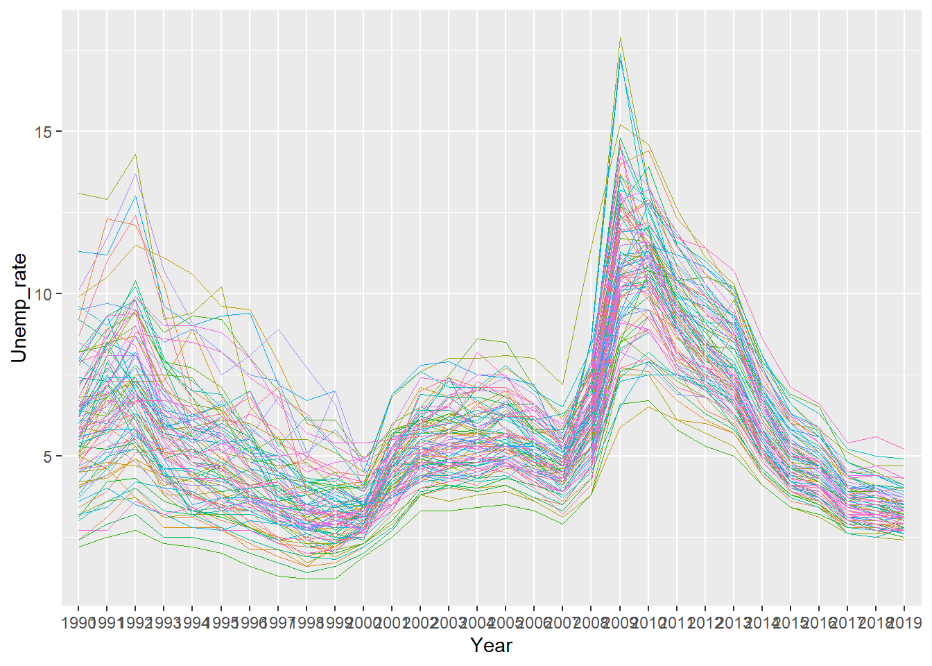

This already is looking a lot better. But can we do something about the labels on the x axis, they are overlaying on each other. We could make the text smaller but then it would be difficult to see, so let’s just rotate them. Also let’s make the y-axis name a bit more meaningful.

ggplot(data=indiana, aes(x=Year, y=Unemp_rate,   # 1
    colour=County_fips, group=County_fips))+     # 2
  geom_line(size=0.3)+                           # 3
  theme(legend.position="none",                  # 4
    axis.text.x=element_text(angle=45)) +        # 5
  ylab('Indiana Unemployment Rate by County')    # 6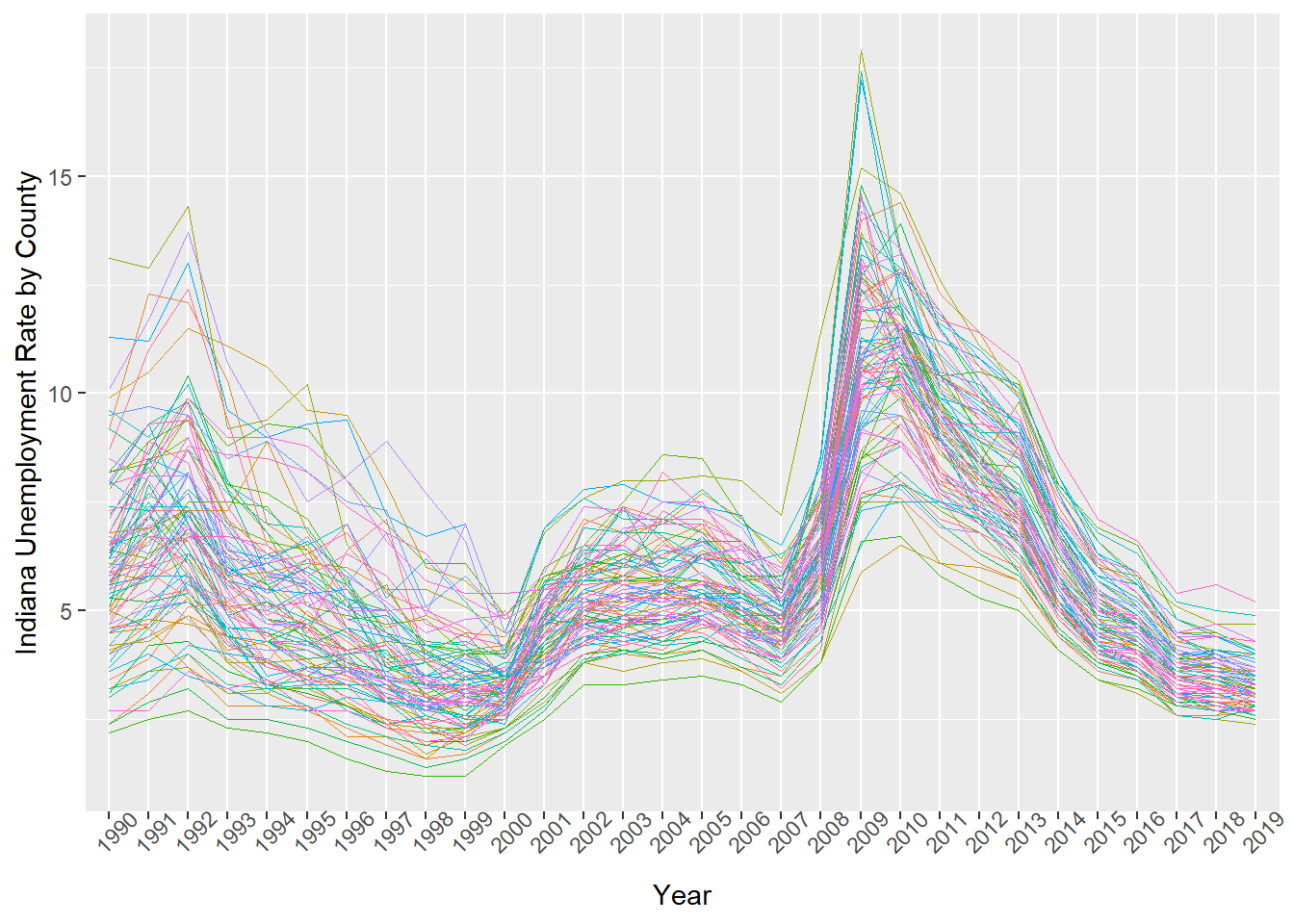

Now we’re getting somewhere! But what if we want to emphasize the county Bloomington is in, Monroe County?

monroecty<-indiana %>% filter(County_fips=="105")       # 1
                                                        # 2
ggplot(data=indiana, aes(x=Year, y=Unemp_rate,          # 3
    colour=County_fips, group=County_fips))+            # 4
  geom_line(size=0.3)+                                  # 5
  geom_line(data=monroecty, aes(x=Year, y=Unemp_rate,   # 6
    colour=County_fips, group=1),                       # 7
    size=0.6, colour='black') +                         # 8
  theme(legend.position="none",                         # 9
    axis.text.x=element_text(angle=45)) +              # 10
  ylab('Indiana Unemployment Rate by County')          # 11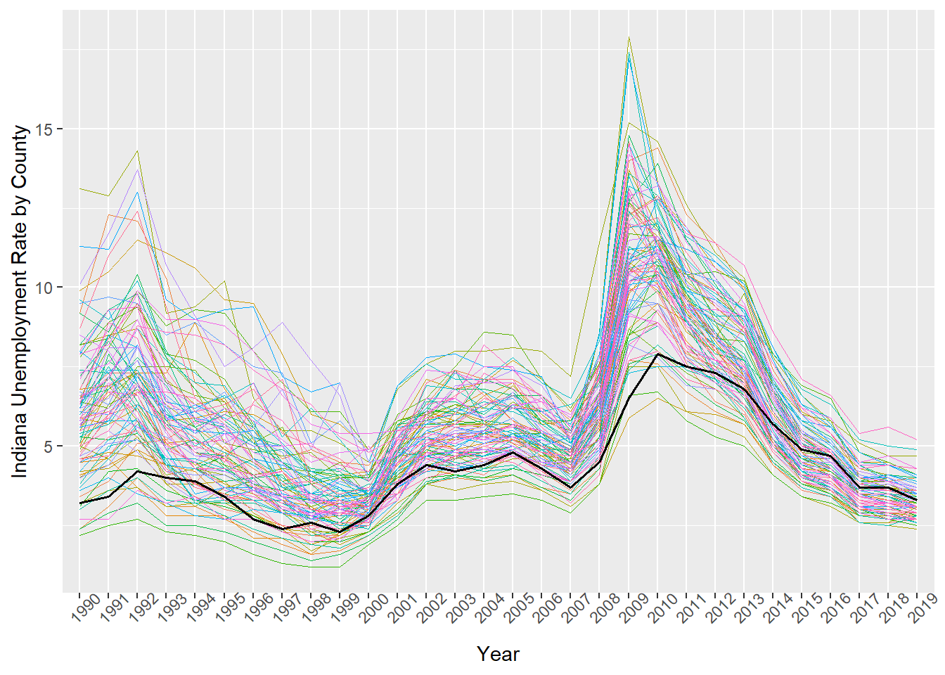

We can make the black line for Monroe County ‘pop’ a bit more too. Let’s change the opacity of the other counties lines. To do this we can set a value, alpha. This takes values 0 to 1 where smaller values are more transparent.

ggplot(data=indiana, aes(x=Year, y=Unemp_rate,          # 1
    colour=County_fips, group=County_fips))+            # 2
  geom_line(size=0.3, alpha=0.5)+                       # 3
  geom_line(data=monroecty, aes(x=Year, y=Unemp_rate,   # 4
    colour=County_fips, group=1),                       # 5
    size=0.6, colour='black') +                         # 6
  theme(legend.position="none",                         # 7
    axis.text.x=element_text(angle=45)) +               # 8
  ylab('Indiana Unemployment Rate by County')           # 9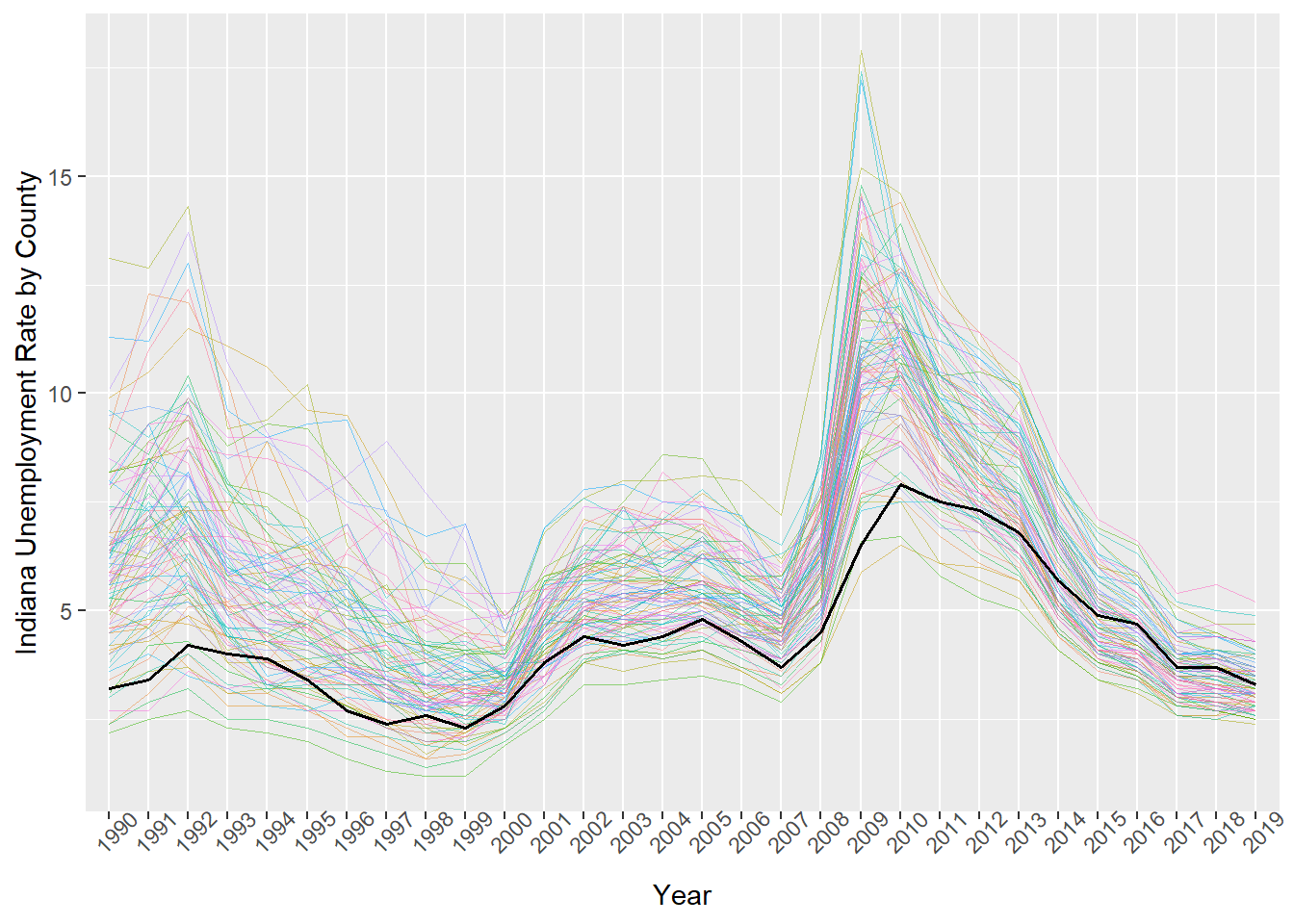

3.2.1 Scatter plot (geom_point)

What if we want points to insteaed of lines for each year?

ggplot(data=indiana, aes(x=Year, y=Unemp_rate,   # 1
  colour=County_fips, group=County_fips))+       # 2
  geom_point()                                   # 3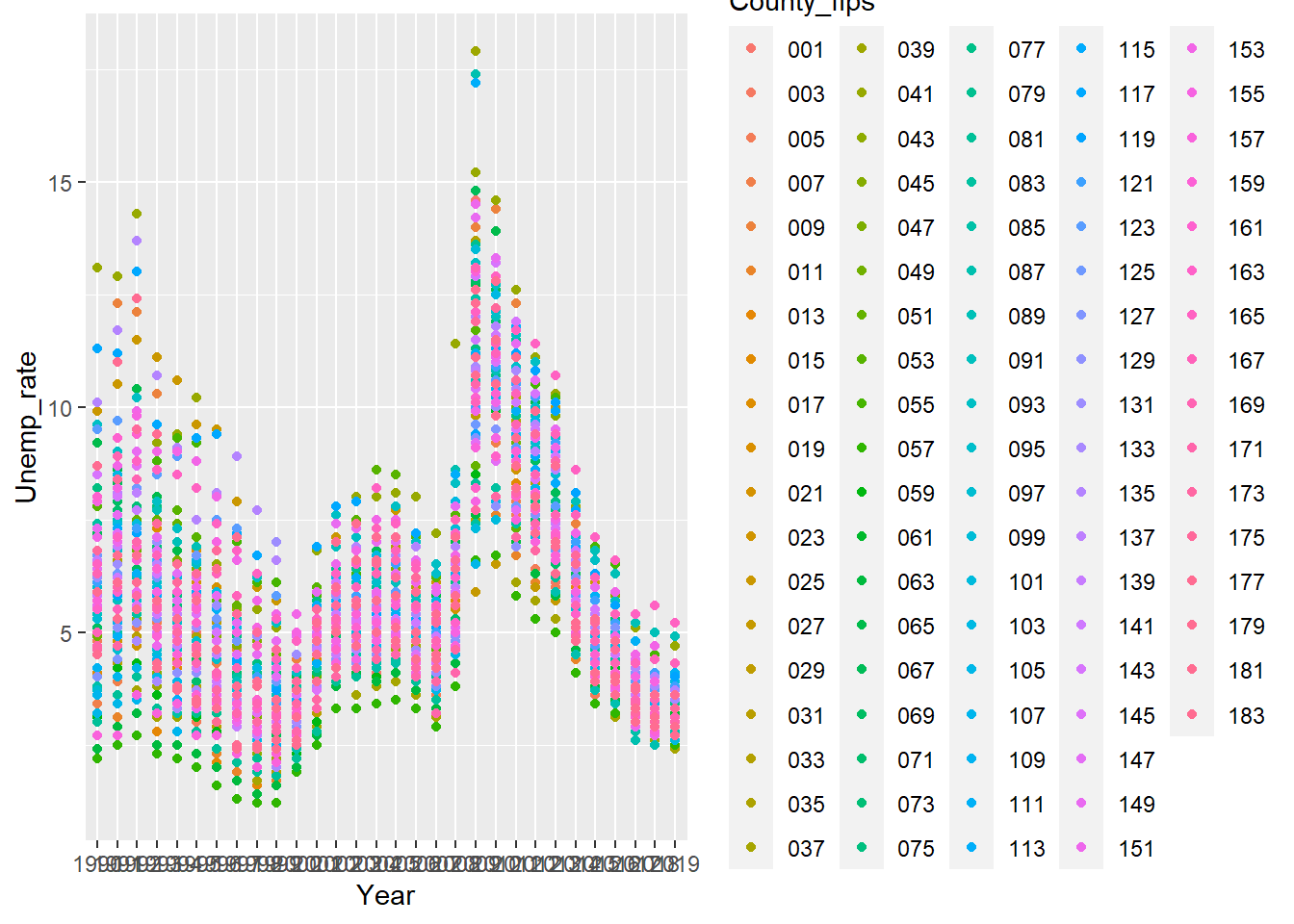

3.3 Manipulating within Groups

Our next chunk of code gets a bit more complex, let’s take it peice by peice though.

  indiana %>% group_by(Year) %>%          # 1
    summarise(Average=mean(Labor_force))  # 2

Let’s again take it from the end and work our ways backwards through it. The 3rd line above is calculating a new variable within a group that is called ‘Average.’ The group (line 2) that we are calculating within is each Year for our Indiana data.frame. That is this snippet of code will give us one value back for each year, the average Labor Force level across Indiana’s counties.

Year	Average
1990	30593.65
1991	30357.00
1992	31058.60
1993	32046.84
1994	33308.01
1995	34078.00
1996	33800.80
1997	33919.72
1998	33947.47
1999	33965.91
2000	33982.50
2001	34140.32
2002	34469.34
2003	34597.76
2004	34432.72
2005	34841.75
2006	35164.35
2007	34866.21
2008	35131.49
2009	34717.45
2010	34512.97
2011	34586.91
2012	34454.88
2013	34656.59
2014	35052.00
2015	35508.30
2016	36178.11
2017	36243.96
2018	36756.59
2019	36819.25

This group_by command paired with summarise is quite useful. For example going back to our original data.frame, county_data. Suppose we wanted to do what we just did but for all states. That is calculate within each state and year combination. With the group_by command this is quite simple! (I print the first 100 lines of output below)

unemp_data %>%                          # 1
  group_by(Year, State_fips) %>%        # 2
  summarise(Average=mean(Labor_force))  # 3

## `summarise()` has grouped output by 'Year'. You can override using the `.groups` argument.

Year	State_fips	Average
1990	01	28468.343
1990	02	10323.923
1990	04	119079.067
1990	05	15091.147
1990	06	261007.414
1990	08	27557.641
1990	09	227471.000
1990	10	120074.667
1990	11	328924.000
1990	12	96480.269
1990	13	20653.579
1990	15	137730.500
1990	16	11193.045
1990	17	58304.049
1990	18	30593.652
1990	19	14664.212
1990	20	12119.305
1990	21	14619.667
1990	22	29216.547
1990	23	39563.625
1990	24	107919.000
1990	25	229027.357
1990	26	55509.072
1990	27	27573.690
1990	28	14438.854
1990	29	22737.852
1990	30	7198.929
1990	31	8871.215
1990	32	39407.176
1990	33	62009.100
1990	34	193117.000
1990	35	21630.061
1990	36	142149.565
1990	37	34765.130
1990	38	5985.226
1990	39	61586.670
1990	40	19786.338
1990	41	41408.833
1990	42	86992.045
1990	44	105072.600
1990	45	37903.326
1990	46	5260.303
1990	47	25207.768
1990	48	33932.858
1990	49	28352.138
1990	50	21768.214
1990	51	24452.541
1990	53	64751.974
1990	54	13857.600
1990	55	35970.542
1990	56	10259.348
1990	72	14517.090
1991	01	28665.134
1991	02	10626.000
1991	04	120334.200
1991	05	15060.213
1991	06	260801.552
1991	08	28035.766
1991	09	230137.750
1991	10	120571.333
1991	11	321433.000
1991	12	97499.104
1991	13	20619.044
1991	15	142897.250
1991	16	11547.432
1991	17	58277.431
1991	18	30357.000
1991	19	14896.960
1991	20	12190.105
1991	21	14689.508
1991	22	29804.094
1991	23	40318.625
1991	24	109023.333
1991	25	228211.357
1991	26	55369.482
1991	27	27903.586
1991	28	14439.512
1991	29	23000.835
1991	30	7247.179
1991	31	8992.527
1991	32	41338.118
1991	33	61429.900
1991	34	193610.571
1991	35	21974.485
1991	36	140985.613
1991	37	35380.200
1991	38	5947.509
1991	39	61726.409
1991	40	19575.922
1991	41	42135.556
1991	42	87390.030
1991	44	103603.400
1991	45	38234.348
1991	46	5303.182
1991	47	25407.611
1991	48	34512.854
1991	49	29390.414
1991	50	21683.857
1991	51	25107.677
1991	53	65281.667

Average is just one statistic we may want to calculate, how about percentiles, minimum, maximum, standard deviation. our summarise command will accept more than one argument, we just have to separate by a comma. Let’s also save this as a new data.frame for use in future lessons.

indiana_laborforce<-                       # 1
  indiana %>% group_by(Year) %>%           # 2
  summarise(Min=min(Labor_force),          # 3
    p10th=quantile(Labor_force, c(0.1)),   # 4
    p25th=quantile(Labor_force, c(0.25)),  # 5
    p50th=quantile(Labor_force, c(0.5)),   # 6
    p75th=quantile(Labor_force, c(0.75)),  # 7
    p90th=quantile(Labor_force, c(0.9)),   # 8
    Max=max(Labor_force),                  # 9
    Average=mean(Labor_force),            # 10
    StDev=sd(Labor_force))                # 11

Year	Min	p10th	p25th	p50th	p75th	p90th	Max	Average	StDev
1990	2629	6639.3	9617.50	14858.5	30089.50	60784.5	424053	30593.65	52989.19
1991	2541	6380.5	9480.00	14713.0	30131.00	62309.9	421789	30357.00	52670.08
1992	2550	6284.2	9615.50	15169.5	31117.00	63623.2	429239	31058.60	53551.02
1993	2607	6200.6	10037.75	15652.5	32034.75	64549.9	438377	32046.84	54683.97
1994	2681	6453.1	10480.50	16472.0	33808.25	66506.3	453457	33308.01	56427.35
1995	2714	6543.2	10994.75	16648.5	34588.00	67364.5	459603	34078.00	57219.27
1996	2724	6522.6	10827.50	16551.0	34597.25	66487.5	453728	33800.80	56670.37
1997	2698	6585.3	10966.00	16671.5	34786.50	66195.3	453928	33919.72	56870.28
1998	2701	6629.7	11008.75	16660.0	34150.50	65887.6	452412	33947.47	56827.82
1999	2691	6496.7	10986.75	16958.5	33968.50	65196.0	448732	33965.91	56434.89
2000	2985	7053.5	10816.50	16984.5	34996.50	63718.6	455135	33982.50	56818.02
2001	2982	7085.7	10709.00	17127.5	34674.75	64832.0	459505	34140.32	57318.59
2002	3051	7040.7	10802.75	17244.5	34974.75	66572.3	462330	34469.34	57807.67
2003	3092	6941.0	10709.50	17199.0	34514.75	67751.5	464331	34597.76	58056.22
2004	3109	6815.2	10547.00	17083.5	33431.50	68476.2	459140	34432.72	57583.09
2005	3152	7075.8	10702.75	17357.5	33606.00	69985.6	459492	34841.75	57925.42
2006	3107	6883.1	10620.50	17326.5	34554.50	72792.0	461468	35164.35	58484.53
2007	3026	6816.7	10447.50	16881.0	34304.50	73128.1	460046	34866.21	58342.88
2008	3044	6816.2	10488.00	16673.5	34065.50	75072.0	463200	35131.49	58819.13
2009	3088	6758.4	10434.25	16452.0	33700.25	74434.1	457524	34717.45	58083.80
2010	3263	6440.5	10308.00	16622.0	33921.75	74406.0	452836	34512.97	57806.16
2011	3210	6459.9	10184.25	16630.5	33804.00	75620.5	456011	34586.91	58199.53
2012	3181	6336.2	10058.50	16453.0	32924.00	76458.0	458377	34454.88	58388.80
2013	3165	6325.9	9900.50	16289.5	33053.00	78149.5	463346	34656.59	58983.65
2014	3216	6401.2	9851.50	16524.0	33215.50	80113.3	467169	35052.00	59579.47
2015	3178	6341.8	9924.75	16908.0	33960.00	82327.7	472330	35508.30	60275.44
2016	3226	6444.8	9930.50	17093.5	35149.00	85223.0	481434	36178.11	61517.07
2017	3153	6512.5	9783.75	17119.0	35516.50	85487.6	483607	36243.96	61840.36
2018	3189	6561.9	9943.50	17334.5	36211.00	86905.8	488698	36756.59	62659.34
2019	3201	6615.6	9812.75	17243.0	36470.50	87146.9	492967	36819.25	63114.77

3.4 Defining New Variables

How about if we don’t want to calculate summary statistics within a group, but just want to calculate a new variable from each observation? Consider if we had unemployed and labor force levels but did not have unemployment rate, how could we go about calculating it with mutate?

indiana<-                                                                # 1
  indiana %>%                                                            # 2
  mutate(unemp_rate_calc=round((Unemployed/Labor_force)*100, digits=1))  # 3

Note since we are defining our new data frame as indiana, the one we are manipulating, we are in this case overwriting the indiana data.frame. Since the unemployment rate in our file was listed as percent and rounded to the nearest tenth, I did the same for our calculated. (digits=1 means one decimal place)

Now let’s compare the first rows of the given unemployment rate with the one we just calculated.

## # A tibble: 6 x 2
##   Unemp_rate unemp_rate_calc
##        <dbl>           <dbl>
## 1        6.5             6.5
## 2        5.1             5.1
## 3        4.8             4.8
## 4        3.4             3.4
## 5        9.2             9.2
## 6        2.4             2.4

3.5 Dropping Variables

How can we go about dropping or keeping certain variables?

Say we wanted to drop the unemp_rate_calc, Labor_force, and Employed?

temp<-                                                 # 1
  indiana %>%                                          # 2
  select(-c(unemp_rate_calc, Labor_force,  Employed))  # 3
head(temp)                                             # 4

## # A tibble: 6 x 7
##   LAUS_code       State_fips County_fips County_name            Year  Unemployed Unemp_rate
##   <chr>           <chr>      <chr>       <chr>                  <chr>      <dbl>      <dbl>
## 1 CN1800100000000 18         001         Adams County, IN       1990         998        6.5
## 2 CN1800300000000 18         003         Allen County, IN       1990        8317        5.1
## 3 CN1800500000000 18         005         Bartholomew County, IN 1990        1632        4.8
## 4 CN1800700000000 18         007         Benton County, IN      1990         156        3.4
## 5 CN1800900000000 18         009         Blackford County, IN   1990         643        9.2
## 6 CN1801100000000 18         011         Boone County, IN       1990         483        2.4

Now what if we wanted to keep just State_fips, County_fips, Year, and Unemp_rate?

temp<-                                                  # 1
  indiana %>%                                           # 2
  select(c(State_fips, County_fips, Year, Unemp_rate))  # 3
head(temp)                                              # 4

## # A tibble: 6 x 4
##   State_fips County_fips Year  Unemp_rate
##   <chr>      <chr>       <chr>      <dbl>
## 1 18         001         1990         6.5
## 2 18         003         1990         5.1
## 3 18         005         1990         4.8
## 4 18         007         1990         3.4
## 5 18         009         1990         9.2
## 6 18         011         1990         2.4

That is if we include the “-” before our variables, we are telling dplyr through our select argument to drop the variables we list. While if we don’t have the “-,” we are telling dplyr to keep only these variables.

3.6 Merging Datasets

What if we have 2 data sets, both county level. How could we combine them?

3.6.1 Poverty Estimates

We will be merging poverty estimates for the US counties in 2019. A table prepared by the USDA can be found on their website here. Let’s download this and put it into our original_data folder. Now let’s open it and see what the data looks like. One of the first things we can notice is the first 2 lines, United States and Alabama. That is there is county and state level observations in addition to the county level ones. We need to keep this in mind before we merge with our unemployment data.

Try to figure out how to read this data into R by yourself. If you need to review, go back to Downloading/Reading Data. Remember using R Studio to assist with this is probably the simplest way until we get very comfortable with the commands.

Here is the command I use for it:

PovertyEstimates <-                                             # 1
  read_excel(paste0(folder_raw_data, "/PovertyEstimates.xls"),  # 2
  skip = 4)                                                     # 3

Make sure we also have our county unemployment data read in. We can observe both of these data.frames now. The way I would clean this data is the following (of course depends on the question/results you are trying to obtain):

• unemployment data:
  1. restrict to 2019 data (as our other county data is just 2019)
  2. Drop Year variable (as we only have one year now)
  3. Drop Puerto Rico (State FIPS 72)
  4. combine state_fips and county_fips into a FIPStxt variable (this is a variable in our poverty data which we will later be using as an ID to merge data on.)
• poverty data:
  1. filter out state/country level observations, leaving just county level.

Here is the code I use for this:

unem_2019<-county_data %>%                                                            # 1
  filter(Year==2019, State_fips!=72) %>% #restrict sample to only year 2019, drop PR  # 2
  select(-Year) %>% #drop the variable Year                                           # 3
  mutate(FIPStxt=paste0(State_fips, County_fips)) #Create variable to merge on        # 4
                                                                                      # 5
pov_2019 <- PovertyEstimates %>%                                                      # 6
  filter(substr(FIPStxt, str_length(FIPStxt)-2, str_length(FIPStxt))!="000")          # 7

Now if we observe both data frames we are left with what we want to merge. We have defined a variable FIPStxt which we would like to join observations on. That is for a given FIPStxt ID in our unemployment data, we would like to find the row with that FIPStxt ID in our poverty data, then add the variables in the poverty data to our unemployment data. Then do this for all iterations of our FIPStxt ID.

There are join commands for this in the dplyr package. The clearest join command is full_join. This matches data frames based on common variable names (or defined variable names to match on.) I print the first 3 rows below.

clean_full<-                         # 1
  unem_2019 %>% full_join(pov_2019)  # 2

## Joining, by = "FIPStxt"

LAUS_code	State_fips	County_fips	County_name	Labor_force	Employed	Unemployed	Unemp_rate	FIPStxt	Stabr	Area_name	Rural-urban_Continuum_Code_2003	Urban_Influence_Code_2003	Rural-urban_Continuum_Code_2013	Urban_Influence_Code_2013	POVALL_2019	CI90LBALL_2019	CI90UBALL_2019	PCTPOVALL_2019	CI90LBALLP_2019	CI90UBALLP_2019	POV017_2019	CI90LB017_2019	CI90UB017_2019	PCTPOV017_2019	CI90LB017P_2019	CI90UB017P_2019	POV517_2019	CI90LB517_2019	CI90UB517_2019	PCTPOV517_2019	CI90LB517P_2019	CI90UB517P_2019	MEDHHINC_2019	CI90LBINC_2019	CI90UBINC_2019	POV04_2019	CI90LB04_2019	CI90UB04_2019	PCTPOV04_2019	CI90LB04P_2019	CI90UB04P_2019
CN0100100000000	01	001	Autauga County, AL	26172	25458	714	2.7	01001	AL	Autauga County	2	2	2	2	6723	5517	7929	12.1	9.9	14.3	2040	1472	2608	15.9	11.5	20.3	1376	902	1850	14.4	9.4	19.4	58233	52517	63949	NA	NA	NA	NA	NA	NA
CN0100300000000	01	003	Baldwin County, AL	97328	94675	2653	2.7	01003	AL	Baldwin County	4	5	3	2	22360	18541	26179	10.1	8.4	11.8	6323	4521	8125	13.5	9.6	17.4	4641	3295	5987	13.3	9.4	17.2	59871	54593	65149	NA	NA	NA	NA	NA	NA
CN0100500000000	01	005	Barbour County, AL	8537	8213	324	3.8	01005	AL	Barbour County	6	6	6	6	5909	4787	7031	27.1	22.0	32.2	2050	1560	2540	41.0	31.2	50.8	1468	1114	1822	39.5	30.0	49.0	35972	31822	40122	NA	NA	NA	NA	NA	NA

3.6.2 left_join

While the above full_join command is probably the ‘safest’ route since it prints all of the variables and rows of both data frames, knowing more about other joins can save us some time.

For example, consider above when we first loaded in our poverty data. It had observations at state and country wide levels in addition to the county level data we wanted. We would ideally want a command that took in the county unemployment data, matched the poverty data based on FIPStxt, and then just exclude any extras from the poverty data. We can do this with left (or right) join.

unclean_left<-                               # 1
  unem_2019 %>% left_join(PovertyEstimates)  # 2

## Joining, by = "FIPStxt"

LAUS_code	State_fips	County_fips	County_name	Labor_force	Employed	Unemployed	Unemp_rate	FIPStxt	Stabr	Area_name	Rural-urban_Continuum_Code_2003	Urban_Influence_Code_2003	Rural-urban_Continuum_Code_2013	Urban_Influence_Code_2013	POVALL_2019	CI90LBALL_2019	CI90UBALL_2019	PCTPOVALL_2019	CI90LBALLP_2019	CI90UBALLP_2019	POV017_2019	CI90LB017_2019	CI90UB017_2019	PCTPOV017_2019	CI90LB017P_2019	CI90UB017P_2019	POV517_2019	CI90LB517_2019	CI90UB517_2019	PCTPOV517_2019	CI90LB517P_2019	CI90UB517P_2019	MEDHHINC_2019	CI90LBINC_2019	CI90UBINC_2019	POV04_2019	CI90LB04_2019	CI90UB04_2019	PCTPOV04_2019	CI90LB04P_2019	CI90UB04P_2019
CN0100100000000	01	001	Autauga County, AL	26172	25458	714	2.7	01001	AL	Autauga County	2	2	2	2	6723	5517	7929	12.1	9.9	14.3	2040	1472	2608	15.9	11.5	20.3	1376	902	1850	14.4	9.4	19.4	58233	52517	63949	NA	NA	NA	NA	NA	NA
CN0100300000000	01	003	Baldwin County, AL	97328	94675	2653	2.7	01003	AL	Baldwin County	4	5	3	2	22360	18541	26179	10.1	8.4	11.8	6323	4521	8125	13.5	9.6	17.4	4641	3295	5987	13.3	9.4	17.2	59871	54593	65149	NA	NA	NA	NA	NA	NA
CN0100500000000	01	005	Barbour County, AL	8537	8213	324	3.8	01005	AL	Barbour County	6	6	6	6	5909	4787	7031	27.1	22.0	32.2	2050	1560	2540	41.0	31.2	50.8	1468	1114	1822	39.5	30.0	49.0	35972	31822	40122	NA	NA	NA	NA	NA	NA

In this case we are starting with our unemployment data, and then telling R to match all possible values by our common variable (FIPStxt here), then we don’t care about any poverty estimate observations that can’t be matched. However what about unemployment observations that can’t be? We simply fill these values with NA’s. For example, if we DON’T exclude Puerto Rico, it would be in our unemployment data, but not in our poverty data. Let’s see what happens:

unem_2019_pr<-county_data %>%                      # 1
  filter(Year==2019) %>%                           # 2
  select(-Year) %>%                                # 3
  mutate(FIPStxt=paste0(State_fips, County_fips))  # 4
pr<-                                               # 5
  unem_2019_pr %>%                                 # 6
  left_join(PovertyEstimates) %>%                  # 7
  filter(State_fips==72)                           # 8

## Joining, by = "FIPStxt"

LAUS_code	State_fips	County_fips	County_name	Labor_force	Employed	Unemployed	Unemp_rate	FIPStxt	Stabr	Area_name	Rural-urban_Continuum_Code_2003	Urban_Influence_Code_2003	Rural-urban_Continuum_Code_2013	Urban_Influence_Code_2013	POVALL_2019	CI90LBALL_2019	CI90UBALL_2019	PCTPOVALL_2019	CI90LBALLP_2019	CI90UBALLP_2019	POV017_2019	CI90LB017_2019	CI90UB017_2019	PCTPOV017_2019	CI90LB017P_2019	CI90UB017P_2019	POV517_2019	CI90LB517_2019	CI90UB517_2019	PCTPOV517_2019	CI90LB517P_2019	CI90UB517P_2019	MEDHHINC_2019	CI90LBINC_2019	CI90UBINC_2019	POV04_2019	CI90LB04_2019	CI90UB04_2019	PCTPOV04_2019	CI90LB04P_2019	CI90UB04P_2019
CN7200100000000	72	001	Adjuntas Municipio, PR	4115	3485	630	15.3	72001	NA	NA	NA	NA	NA	NA	NA	NA	NA	NA	NA	NA	NA	NA	NA	NA	NA	NA	NA	NA	NA	NA	NA	NA	NA	NA	NA	NA	NA	NA	NA	NA	NA
CN7200300000000	72	003	Aguada Municipio, PR	11743	10553	1190	10.1	72003	NA	NA	NA	NA	NA	NA	NA	NA	NA	NA	NA	NA	NA	NA	NA	NA	NA	NA	NA	NA	NA	NA	NA	NA	NA	NA	NA	NA	NA	NA	NA	NA	NA
CN7200500000000	72	005	Aguadilla Municipio, PR	14350	12881	1469	10.2	72005	NA	NA	NA	NA	NA	NA	NA	NA	NA	NA	NA	NA	NA	NA	NA	NA	NA	NA	NA	NA	NA	NA	NA	NA	NA	NA	NA	NA	NA	NA	NA	NA	NA

3.6.3 Additional Resources

In addition to full and left join shown here, there is also inner join and right join. Details of these can be found here.