2 Introduction
The goal of this section is to provide a very quick introduction or refresher to R. If this is your first time coding, this brief introduction will most likely be quite insufficient. I encourage you to seek other resources to learn the basics before proceeding.
In particular we will cover:
- Writing Loops
- String Manipulation
- Project Organization
- Downloading/Reading Data
- Downloading Loop
In this lesson we will be downloading and cleaning data from the BLS on county level employment statistics from 1990-2019.
2.1 Very Basics
I assume you have R installed and running. There are plenty of guides online on how to do this.
Let’s first define some arrays within R.
These can be numeric based, in this case integer.
Let’s dig into what is going on a bit more. We are telling R to define a vector, this is the c( ) part, with elements 1,2,3 and give that vector a name A. The backwards arrow tells R what is the name and what is the element we are defining.
We can make character based vectors as well.
We can then combine these vectors into a dataframe (this is relevant for when we start thinking about reading in/manipulating actual data). Since all of our vectors are length three, we can easily create a dataframe (think a matrix) where our column names will be the name of the vectors, and the rows will be the elements of the vectors.
##   numvec1 numvec2 charvec1 charvec2
## 1       5       7        a        d
## 2       6       8        b        e
## 3       7       9        c        f
Now first_dataframe is going to be of similar format as we will typically have when we read in data from excel files into R. We can access certain rows and columns within the dataframe by putting square brackets after the name of the dataframe. For example if we wanted to print the element in the first row and first column, we could define the variable x as this and then print x. (Keep in mind the ordering is rows, columns)
## [1] 5What if we wanted to print all elements in the first row, we just leave the column (after the comma) blank:
##   numvec1 numvec2 charvec1 charvec2
## 1       5       7        a        d
How about 1st & 3rd row?
##   numvec1 numvec2 charvec1 charvec2
## 1       5       7        a        d
## 3       7       9        c        f
Another way to do this is to define another variable, say y as a vector with elements 1 and 3. Notice how the below output is the same as the above.
##   numvec1 numvec2 charvec1 charvec2
## 1       5       7        a        d
## 3       7       9        c        f
We can do the same thing for the columns (we need to remember the order for the square brackets are rows, columns). Note: if we put a negative sign in front of these commands in the brackets, instead “keeping” certain rows or columns, it means remove! That is if in the below command we have -3, it would be saying REMOVE column 3!
## [1] "a" "b" "c"## numvec1 numvec2 charvec2
## 1 5 7 d
## 2 6 8 e
## 3 7 9 fOur third column is named C, we can also pull this column by referencing it’s name after a dollar sign, such as:
## [1] "a" "b" "c"This may not sound useful now, but think if we have many columns of variables, say wage, hoursworked, fulltime, and hundreds of more. We don’t want to have to find what column number hoursworked is, we can just reference this column name.
2.1.0.1 “And” and “Or” Operators
A couple common operators that we may want to use are “and” and “or” statements. Within R:
- “&” : Our “and” operator
- “|” : Our “or” operator
For example:
first_dataframe[first_dataframe$numvec1>=6 & first_dataframe$numvec2<9,] # 1## numvec1 numvec2 charvec1 charvec2
## 2 6 8 b e
first_dataframe[first_dataframe$numvec1>=6 | first_dataframe$numvec2<9,] # 1## numvec1 numvec2 charvec1 charvec2
## 1 5 7 a d
## 2 6 8 b e
## 3 7 9 c f2.2 Writing Loops
letters<-c("a", "b", "c", "d", "e")  # 1
letters_l<-length(letters)           # 2
for (i in 1:letters_l){              # 3
  print(letters[i])                  # 4
}                                    # 5
## [1] "a"
## [1] "b"
## [1] "c"
## [1] "d"
## [1] "e"Going line by line:
- Line 1: Define a vector of letters.
- Line 2: Report the number of elements in our letter vector and save as letters_l
- Line 3: Defining for loop. Our index will be i, and it will run from 0 to however long letters vector is (try adding some more letters!) Note our for loop action is defined within the curly braces.
- Line 4: For every i defined in Line 3 we want to print the corresponding element in the vector letters.
Okay, great. How does this help us with reading in the data? We’ll get to that in the next section.
2.3 String Manipulation
2.3.1 String Concatenation
## [1] "This is a the startof a sentence"## [1] "This is a the start of a sentence"Notice we define a and b as strings. What paste and paste0 do are combine these strings into one string. We can see that paste places a space between the two strings while paste0 does not. paste0 comes in quite handy for working with file pathing as we will see. Yes it’s that easy!
We will not be using this for this project but it may be useful to know we can concatenate two vectors of strings as well.
a<-c("This is a the start", "Now we have", "This really is", "Economics is")  # 1
b<-c("of a sentence.", "another sentence.", "quite handy.", "awesome!")       # 2
print(paste(a,b))                                                             # 3
## [1] "This is a the start of a sentence." "Now we have another sentence."
## [3] "This really is quite handy." "Economics is awesome!"2.3.2 String Padding
Consider we have a vector of numbers which currently runs 1-19. Now what if we need all the ‘single character’ digits to have a leading zero. That is instead of “1” we need “01.”
We could use paste0 as above and combine a 0 with our vector.
numbvec<-as.character(1:19)  # 1
print(paste0("0", numbvec))  # 2
## [1] "01" "02" "03" "04" "05" "06" "07" "08" "09" "010" "011" "012" "013"
## [14] "014" "015" "016" "017" "018" "019"But we don’t want a leading 0 in front of the double ‘character’ digits (ie We DON’T want “090”). We could break our vector into single character digits and two character digits, manipulate the single character digits, then combine it back in with the double character digits. But there is an easier way: str_pad !
require(stringr)                           # 1
numbvec<-as.character(1:19)                # 2
print(str_pad(numbvec, 2, "left", "0")  )  # 3
## [1] "01" "02" "03" "04" "05" "06" "07" "08" "09" "10" "11" "12" "13" "14" "15" "16"
## [17] "17" "18" "19"Now this looks like what we want! But what is str_pad doing? With str_pad we are telling stringr we want all elements of numbvec to be of length 2. So stringr checks to see if the elements are less than 2 characters, if an element is it adds “0”’s to the left side until it reaches length 2. If it is already length 2, it will leave it alone.
There is many other handy commands to deal with strings in R. These are just a couple of commands we will be using. I will be writing a post with some other handy functions in the coming weeks and will link it here.
2.4 Project Organization
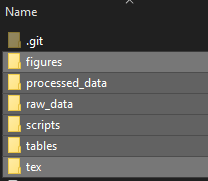
Before we get started, let’s set up a folder for our project and create subfolders to keep things organized. For this project I recommend the following subfolders, which are a good minimum for organizing any project:
- raw_data: This is where we will put our `preprocessed’ data we will be getting from MIT Election Lab.
- scripts: Where we will save all of our R-scripts in this folder
- processed_data: If we want to save some intermediate data steps between raw data and our output.
- tables: Any tex tables we generate we will save to this folder
- figures: Any figures we generate we will save to this folder
- tex: Where we can have our paper and/or presentations
You can make more folders if you feel it keeps you organized. The main point I want to make here is it is well worth your time to think about how you want to organize your project. Oftentimes if we jump right in without a plan, things become a jumbled mess. (If you want to go further with your organization strategies, I recommend looking into waf, specifically check out Templates for Reproducible Research Projects in Economics.)
My project folder now looks like this:
2.4.1 First R script!
Now that we have our folders created, let’s now create paths to those folders with R. Let’s start by creating a variable workingdir which we can define as the path to our main folder.
workingdir<-"PATH_TO_YOUR_WORKING_DIR" # 1Now we are going to create a script, let’s save it as workingdir.R and place it in our main parent folder. We are then going to be using the path we defined above in this script to create paths to our other folders.
folder_figures<-paste0(workingdir, "figures")                # 1
folder_processed_data<-paste0(workingdir, "processed_data")  # 2
folder_raw_data<-paste0(workingdir, "raw_data")              # 3
folder_scripts<-paste0(workingdir, "scripts")                # 4
folder_tables<-paste0(workingdir, "tables")                  # 5
folder_tex<-paste0(workingdir, "tex")                        # 6
Now at the top of all other scripts we can have:
Now all this says is we have a variable named workingdir that points to our main parent folder. We then have a script in which we define paths to all other folders. With this at the front of all of our scripts, we can easily reference them to create easier pathing for ourselves.
2.5 Downloading within R
We can use R to with a direct link to download. The first argument the download.file() command takes that we will use is the url of the xslx document and the second argument is the destination it will be saved. The last argument is basically telling R that the excel docs are not plain text. (Don’t forget to have workingdir defined as we did in Project Organization
download.file("https://www.bls.gov/lau/laucnty90.xlsx",     # 1
  paste0(folder_raw_data, "bls_unemp_90.xlsx"), mode="wb")  # 2
2.6 Reading in Data
Before we read in this data to R, let’s see what we are dealing with. Opening up the file in excel we can see there will be issues reading the file in.
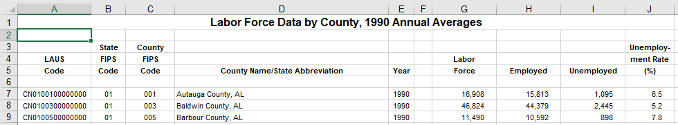
We can notice that the first row has the file title spread across columns A:J. Variable names are spread across anywhere 1-3 rows. And lastly we have an empty column in F. The bright side is if we observe the other year’s files, they all have this exact same structure. Hence we will able to use a loop eventually to clean them all instead of one at a time.
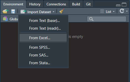
The main package we will be using is readxl, which is quite self explanatory. It is a package meant to help to read in excel docs. Let’s try to open the file for 1990 we downloaded in R. We can do this through R Studio’s functionality.
Within the “Environment” area of R Studio, click Import Dataset, then From Excel…
There is definitely multiple ways to do this, as we can see from the options available. I first deselect “First Row as Names” (This option is very nice if your data is already in a precleaned form and your first row simply has your variable names.) I then begin to skip rows, 5 rows of skipping leads to the first row being the first row of data.
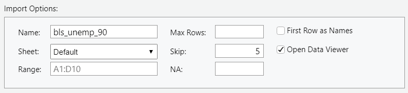
Next we can handle column F that we noticed was blank. This is column 6 and stays consistent across all years (you can check this). Remembering our lessons from the Very Basics section we can subset this dataframe by removing column 6.
Hence we have something that will look like the following for our command for our script.
require(readxl)                                                                           # 1
workingdir<-"C:/Users/weste/Documents/GitHub/r-introtodatascience/sample_repo/"           # 2
bls_unemp_90 <- read_excel(paste0(folder_raw_data, "/bls_unemp_90.xlsx"),                 # 3
                           col_names=FALSE, skip=5)                                       # 4
bls_unemp_90<-bls_unemp_90[,-6]                                                           # 5
colnames(bls_unemp_90)<-c("LAUS_code", "State_fips", "County_fips", "County_name",        # 6
                          "Year", "Labor_force", "Employed", "Unemployed", "Unemp_rate")  # 7
Where the last line above we are giving our columns names based on the names we saw in the excel document.
We can then observe our data frame to ssee if it’s fully cleaned. At first it seems so (I actually initially thought so). However when reading in the data, we grabbed 2 extra rows at the end of the file. Hence we have 2 rows at the end of our data frame that are NA’s. Let’s drop these two rows, to do this we can use a command is.na and prior to it include an “!” saying ‘not is.na.’
bls_unemp_90<-bls_unemp_90[!is.na(bls_unemp_90$State_fips),] # 1Here is a good place to pause if you want a challenge. You should have all the tools needed to write a loop to download all files from 1990-2019.
2.7 Download Loop
In the next sections we will be using county level employment/labor force data from BLS to learn more about working with actual data. We will be using the Labor force data by county, yearly annual averages. There is data from 1990-2019 (as of writing these notes). To start we are going to download this data and then read it into R.
We can use a loop to download/clean our data such as this:
require(stringr)                                                                # 1
require(readxl)                                                                 # 2
unemp_data<-data.frame()                                                        # 3
years<-c(90:99, 0:19)                                                           # 4
years<-str_pad(as.character(years), 2, "left", "0")                             # 5
years_l<-length(years)                                                          # 6
for (i in 1:years_l){                                                           # 7
url<-paste0("https://www.bls.gov/lau/laucnty", years[i], ".xlsx")               # 8
destination<-paste0(folder_raw_data, "/bls_unemp_", years[i], ".xlsx")          # 9
download.file(url, destination, mode="wb")                                     # 10
temp_df <- read_excel(paste0(folder_raw_data, "/bls_unemp_", years[i],         # 11
  ".xlsx"),col_names=FALSE, skip=5)                                            # 12
temp_df<-temp_df[,-6]                                                          # 13
colnames(temp_df)<-c("LAUS_code", "State_fips", "County_fips", "County_name",  # 14
  "Year", "Labor_force", "Employed", "Unemployed", "Unemp_rate")               # 15
temp_df<-temp_df[!is.na(temp_df$State_fips),]                                  # 16
unemp_data<-rbind(county_data, temp_df)                                        # 17
}                                                                              # 18
filename<-paste0(folder_processed_data, "/unemp_data.rda")                     # 19
save(unemp_data, file=filename)                                                # 20
To work through this first let’s think what we are trying to achieve. The links for the downloads are all in the form of https://www.bls.gov/lau/laucntyZZ.xlsx, where ZZ is two digits representing the year. These ZZ values run from “90”to “99” for years 1990-1999 and “00” to “19” for years 2000-2019.
Let’s work through the above code line by line:
- Lines #1 & #2: load required packages.
- Line #3: Declare unemp_data will be a data.frame. Right now it is empty, but we will add to it.
- Line #4: Define a vector with elements 90-99 and 0-19. (Which will correspond to the years that we will pull)
- Line #5 : We have a vector for years, however if we notice in the url names we need this vector to include a leading 0 in front of the single ‘character’ digits (ie “01” instead of “1”). But we don’t want a leading 0 in front of the double ‘character’ digits (ie We DON’T want “090”). Go back to the String Manipulation section if you need to refresh on this.
- Line #6 : Calculate the length of years and save as years_l
- Line #7 : See String Manipulation if defining the for loop does not make sense.
- Line #8 : We are creating the character string for the url for the download link. Since they all take the form of https://www.bls.gov/lau/laucntyZZ.xlsx, we can use one element of our years vector at a time. (See String Manipulation for explanation on paste0)
- Line #9 : This is of similar spirit to line #4, but this is defining the path/filename of the excel file we will save.
- Line #10 : This line is just telling R to download the file at that url, save it to the defined location/name, and to read it as a non-raw text form. (see Downloading/Reading Data if unclear.)
- Lines #11-#16: See Downloading/Reading Data for a direct explanation.
- Line #17: rbind appends data. Hence since all of our data has the same format and has a variable indicating the year, we can simply append.
- Line #19: Create the filepath (to our processed_data folder) where we will save the file, what the file name and type is.
- Line #20: save the combined data to the location/name we defined above.
We now have our data cleaned and saved for our next lesson when we will start to work with it more!